For optimization modelers, the journey to production has always involved tradeoffs. Do you sacrifice the convenience of your local IDE for the power of cloud compute? Do you spend weeks re-architecting code to make it "cloud-ready"? Over the past few years, we've explored different approaches to running Gurobi optimization models in Snowflake, and each solved important problems while pointing toward what optimization teams truly need.
The Evolution: From Containers to Notebooks to ML Jobs
Our first approach involved the use of Snowpark Container Services (SPCS). We demonstrated that Gurobi could run inside Snowflake by containerizing optimization workloads with Docker, enabling long-running services and custom runtime environments. This approach gave teams full control over their optimization infrastructure, but required Docker expertise, service management, and architectural decisions around APIs and endpoints, complexity that made sense for sophisticated use cases but felt like overhead for simpler optimization workflows.
Next came Snowflake Notebooks, which transformed optimization into an interactive, collaborative experience. Stakeholders could adjust parameters, re-run analyses, and visualize results without leaving their browser. This was perfect for exploratory work and presenting results to business teams. However, notebooks tied you to the web interface; this is great for collaboration, but limiting when you wanted the full power of VS Code, PyCharm, or your preferred local development environment with debugging and your familiar workflow.
The gap was clear: optimization modelers needed to develop locally with their tools of choice while executing on Snowflake's compute, without re-architecting their code.
Why Snowflake ML Jobs
Snowflake ML Jobs delivers what optimization teams have been looking for: true lift-and-shift simplicity. Write your optimization model once in Python, test it locally with your favorite IDE, then deploy it to Snowflake compute. The same model that runs on your laptop can execute at scale on Snowflake infrastructure.
ML Jobs offers three submission methods: `submit_file()` for single Python scripts, `submit_directory()` for multi-file projects submitted directly from your local machine, and `submit_from_stage()` for code uploaded to Snowflake stages. Each method handles dependency installation, execution environment setup, and result management automatically.
Building a Portfolio Optimization Model
Let's see this in action with a financial portfolio optimization example. The goal is to construct an optimal investment portfolio that maximizes expected returns while respecting real-world constraints: a total budget limit, diversification requirements, and minimum investment thresholds per asset. This is a linear programming problem that financial institutions can utilize daily when rebalancing portfolios.
The optimization reads historical asset data (tickers, expected returns, prices) and constraint parameters from Snowflake tables. Gurobi then solves for the optimal number of shares to purchase for each asset, maximizing the portfolio's total expected return subject to all constraints. Results, including asset allocations, investment amounts, and portfolio percentages, are written back to Snowflake tables for reporting and analysis.
The `PortfolioOptimizer` class encapsulates this entire workflow. It loads data using Snowpark DataFrames, creates Gurobi decision variables for share quantities, defines the objective function (maximize total expected return), and adds constraints for budget limits and diversification rules. After solving, it formats results as DataFrames and writes them back to Snowflake using Snowpark's `write.save_as_table()` method. The class is designed to work identically whether data comes from Snowflake tables or local CSV files, making it easy to develop and test locally before deploying.
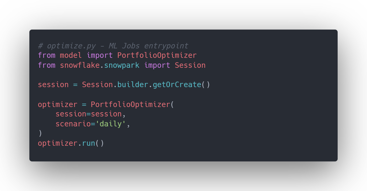
The implementation centers around `optimize.py` which is the entrypoint script that ML Jobs will execute. This script creates a Snowpark session, instantiates the optimizer, and runs the complete workflow (Figure 1):
Deploying to Snowflake
Deployment is where ML Jobs shines. After running your Snowflake setup script to create compute pools, stages, and tables, you submit your optimization model with just a few lines. Note that `submit_file()`, `submit_directory()`, and `submit_from_stage()` all share similar parameters including `compute_pool`, `stage_name`, `entrypoint`, `pip_requirements`, `external_access_integrations.` This making it straightforward to choose depending on your use case (Figure 2):
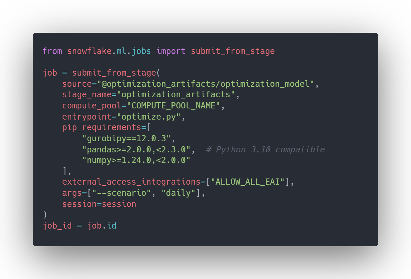
Your optimization now runs on Snowflake compute pools. You can choose from CPU_X64 instances (1-28 vCPUs, 6-116 GB memory) or HIGHMEM instances (up to 240 GB memory) based on your model's requirements. The compute pool provides the horsepower for complex optimizations while Snowflake handles infrastructure, dependency installation, and result storage.
Productionizing with Snowflake Tasks
Running optimization models interactively is useful for development, but production workloads need automation. In the case of a portfolio optimization model, it is typical that analysis runs daily before market opens. This is where Snowflake Tasks become essential; they provide native orchestration to schedule and chain multiple steps into automated workflows without external schedulers.
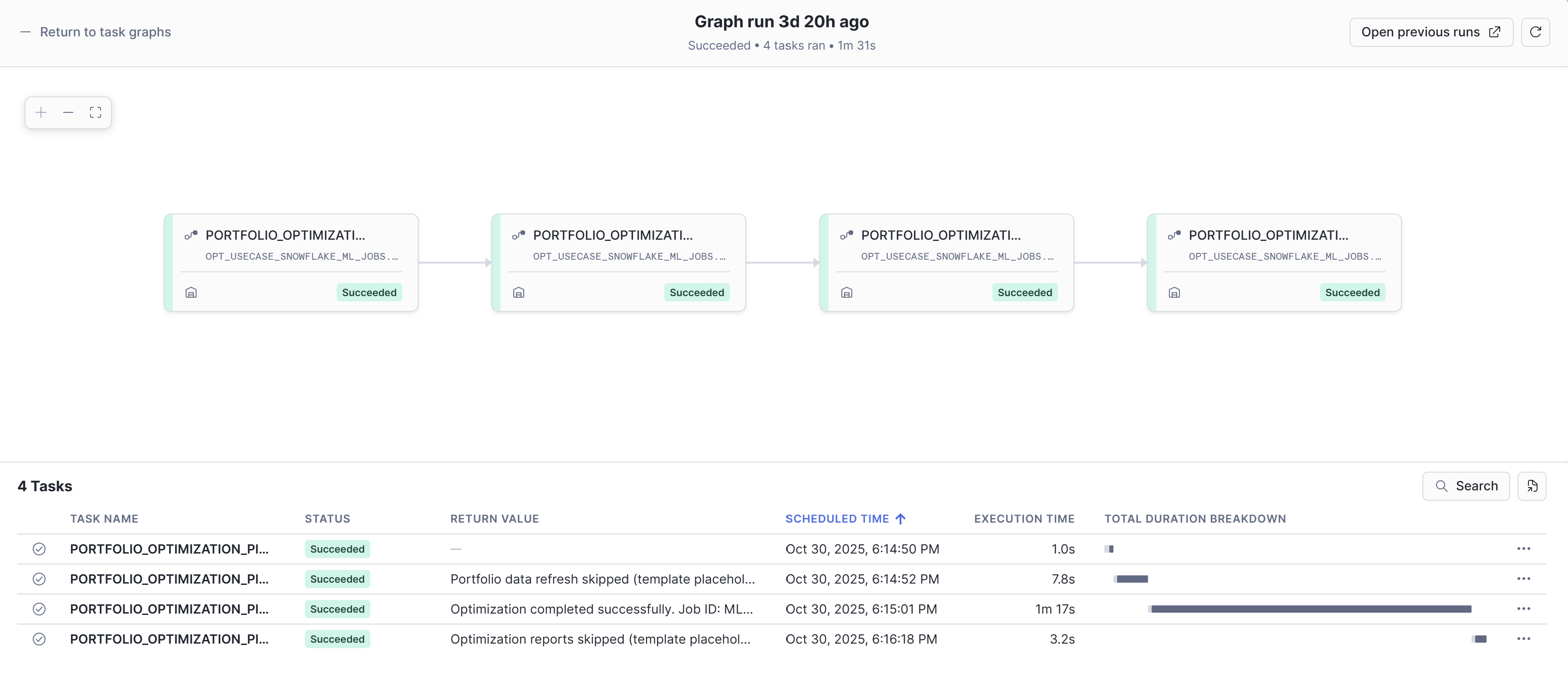
The key insight is that Tasks and ML Jobs work together seamlessly. You define Task functions that call `submit_from_stage()` to launch ML Jobs, then orchestrate those Tasks into a DAG (Directed Acyclic Graph). This lets you build end-to-end pipelines: refresh input data from market feeds, execute the optimization via ML Jobs on compute pools, then generate reports for stakeholders, all running on your desired schedule.
For this integration, `submit_from_stage()` is required because Tasks execute within Snowflake's infrastructure and can't access your local filesystem. Your model files must be uploaded to a stage first, then your Task functions reference that stage location when submitting jobs. Here's a complete DAG for the portfolio optimization pipeline (Figure 3):
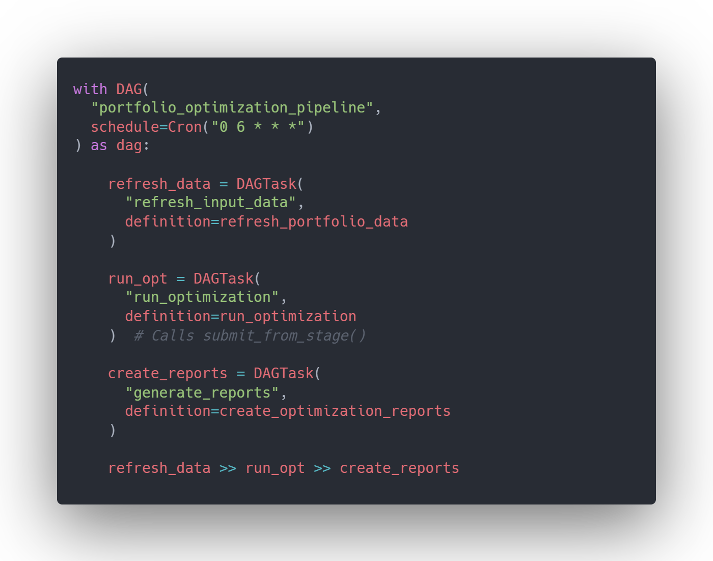
This template pattern works for any optimization model. The DAG structure remains the same; you can customize your data preparation, model parameters, and reporting logic.
Want to try this yourself? Download the complete portfolio optimization codebase template, including the PortfolioOptimizer class, setup scripts, and Task DAG definitions, to adapt for your own optimization use cases.
When to Use Each Approach
Each approach we've explored has its place. Snowflake Notebooks excel for interactive analysis, stakeholder collaboration, and rapid prototyping. SPCS is ideal for custom long-running services and advanced containerized workflows. ML Jobs is perfect for production optimization pipelines where you want local development flexibility with Snowflake's scale and the simplicity of lift-and-shift deployment.
The lift-and-shift promise of ML Jobs means you can maintain your preferred development workflow - version control, local testing, familiar tools - while leveraging Snowflake's computational power and data gravity. No Docker files, no API layers, no code rewrites. Just your optimization model, deployed at scale.
Ready to Streamline Your Optimization Workflows?
Ready to streamline your optimization workflows? Reach out to Aimpoint Digital to discuss implementing Snowflake ML Jobs for your optimization use cases. Whether you're tackling portfolio optimization, supply chain planning, or resource allocation, we can help you develop locally, execute at scale, and productionize seamlessly.